Interferometric calibration of a deformable mirror
For citeable PDF versions of this document, please use the links below.
- DOI (concept): https://doi.org/10.5281/zenodo.3714951
- Authors: Jacopo Antonello, Jingyu Wang, Chao He, Mick Phillips, Martin Booth
- Licence: CC-BY-4.0
- Last modified: 5 yrs ago
The listed authors have participated in the writing of this document. As the content is the culmination of long term work in the Dynamic Optics and Photonics Group, many others have contributed directly or indirectly to this material. We consciously acknowledge all of these contributions, even though it is impractical to list them all here
Abstract
This tutorial discusses the static calibration of a deformable mirror using a Twyman--Green interferometer setup, combined with single-frame fringe analysis for phase extraction. We provide a reference implementation for this method in the form of a toolbox written in Python. In addition, we include detailed instructions to build a compact, slot-in interferometer. This protocol, accompanying software, and hardware design facilitate calibration of deformable mirrors for a range of applications.
Introduction
Deformable mirrors (DM) are devices that impress a controllable wavefront profile on a beam of light upon reflection. Such devices are particularly useful in microscopy applications, where they allow both engineering of the point-spread function and correction of aberrations in an instrument. Once a DM is deployed in an optical path, it must be calibrated so that the desired wavefront modulation can be attained. In this tutorial we describe in detail how to carry out the calibration procedure using an interferometer.
Deformable mirrors have been manufactured using different technologies, each exhibiting its own advantages and inconveniences with respect to individual applications [1; 2]. For example, DMs based on piezoelectric actuation typically feature larger stroke and less inter-actuator coupling with respect to electrostatically actuated DMs. Nevertheless, the former ones suffer from non-linear effects such as hysteresis and creep, which render them unsuitable for open-loop control, as required for wavefront sensorless adaptive optics [3]. Here we only consider DMs that are free of such non-linear effects.
Despite heterogeneity in the underlying technology, virtually all DMs comprise a number of reflective segments or a continuous membrane that can be adaptively manipulated using an array of actuators. Control of a DM therefore consists in choosing which configuration to apply to the actuators in order to obtain a desired shape of the mirror. For this purpose, one must first understand how the active area of the DM responds when actuators are operated. Obtaining this information is the goal of the DM calibration [4; 5].
Is the calibration necessary?
In most scenarios, calibration of the DM is a prerequisite that cannot be neglected if accurate wavefront modulation is sought for a particular application. For example, one may be interested in determining a quantitative estimate of the shape of the DM given a particular arrangement of the actuators. Similarly, calibration is a requirement if one is seeking to optimise the shape of the DM in the most efficient manner possible. For most microscopes, this would entail at least removing some unnecessary degrees of freedom (DOF) such as piston. This latter only affects the mean value of the phase and has no side effects on the quality of the recorded images. Maintaining piston as an active DOF when optimising the shape of the DM does make the optimisation problem more challenging, since it endows this latter with multiple optimal solutions – each exhibiting a different value for the piston. A similar side effect is also encountered if one does not orthogonalise the DOFs that are spanned by the DM actuators, which also leads to a more troublesome optmisation problem. In this case, adjustment of an individual DOF affects the optimal configuration of the other DOFs. Finally, calibration is necessary when seeking control of specific DOFs of interest, such as spherical aberration, which develops when focusing through refractive index mismatches.
On the contrary, there can be scenarios where calibration of the DM is a redundant step. One such example is using the DM to remove time-invariant aberration present in a microscope, such as aberrations due to optical misalignment. In this case, one could optimise the configuration of the actuators directly, for example by running a general model-free optimisation method [3]. As this task must be performed a single time only, it can be successfully completed even in an inefficient manner.
Linear static modelling of the DM
In practical terms, calibration of the DM involves generating a mathematical model \(\Psi\), which explains the relationship between the input control signals \(\mathbf{u}\) applied to the actuators and the corresponding output phase \(\Phi\) imprinted by the DM onto a beam upon reflection,
\[ \begin{equation} \Phi = \Psi(\mathbf{u}). \label{eq:Psiunonlin} \end{equation}\]
In microscopy applications, one can often neglect the dynamical behaviour of the DM and just assume that this latter responds instantaneously to a change in the control signals. Furthermore, one can also assume linearity with respect to \(\mathbf{u}\), which leads to the following simplified model,
\[ \begin{equation} \Phi = \sum \psi_i u_i. \label{eq:Psiulin} \end{equation}\]
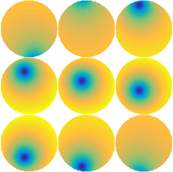
Here \(\psi_i\) represents the influence function of the \(i\)-th actuator. Figure 1 shows a set of typical influence functions recorded when poking different actuators of a DM. It can be seen that the effect of an influence function spreads across the mirror surface and extends over neighbouring actuators.
Figure 1: Influence functions \(\psi\) measured after poking individual actuators of a DM.
When working with experimental data, one has to consider a sampled version of Eq. \eqref{eq:Psiulin}, which leads to
\[ \begin{equation} \boldsymbol{\Phi} = \Psi\mathbf{u}. \label{eq:Psiusamp} \end{equation}\]
Here \(\boldsymbol{\Phi}\) is a vector of size \(N_c\), which represents the phase measured using a wavefront sensor such as a Shack–Hartmann or an interferometer as will be outlined in detail within this tutorial. To see how vector \(\boldsymbol{\Phi}\) is constructed in practice, take one image from Fig. 1 as an example. Since microscopes have circular pupils, one need only consider the pixels within a circular disk called the aperture. The location and size of the aperture with respect to the active area of the DM is determined by the reimaging optics that lie between the microscope back focal plane and the DM. One can take the pixels lying with the aperture, order them with a single index, and finally store them into vector \(\boldsymbol{\Phi}\).
Assuming the DM has \(N_a\) actuators, \(\mathbf{u}\) can also be recognised as a vector and, as a result, one has that \(\Psi\) is an \(N_c \times N_a\) matrix. The columns of \(\Psi\) therefore represent sampled versions of the influence functions \(\psi\). One can estimate matrix \(\Psi\) by recording experimental data in an optical breadboard setup.
Computation of \(\Psi\) using interferometric methods
As discussed above, the first step necessary for the calibration involves measuring \(\Psi\) using an experimental setup. One route to achieve this is via interferometric methods, which are commonly employed for optical testing purposes [6; 7]. One possibility is to use a Twyman–Green interferometer, which is depicted in Fig. 2. Here the DM is placed in the test arm, whereas a flat mirror (FM) is located in the reference arm. Collimated light enters the setup from the bottom edge of a beam splitter (BS) and is split into two beams, one impinging onto the DM and the other onto the flat mirror. After reflection the two beams are recombined by the same BS and imaged onto a camera (CAM). The conjugated planes are indicated by the dashed lines in grey. In particular, it can be seen that the camera plane is conjugated by lens L1 and L2 to the DM and FM.
In principle the DM calibration can be performed once only, and it should not be necessary to repeat it unless something changes in the optical layout. For example, if one shifts the DM laterally within the plane of the mirror, then that results in a change of the position of the actuators with respect to the pupil. The calibration should hence be repeated to account for this new arrangement. It is therefore convenient to be able to repeat the calibration without much effort. One possibility is therefore to include the interferometer in situ, i.e., within microscope setup itself, as a troubleshooting branch. Within the microscope, the DM must be placed in a plane that is conjugate to the back focal plane of the microscope objective (BFP), which is indicated in Fig. 2 by lenses L3 and L4. Note that care should be taken to match the lengths of the reference and test arms if a short coherence light source is used.
As a less convenient alternative, one can build a compact, slot-in interferometer. This latter can be temporarily inserted into the microscope setup in front of the DM to perform the calibration or for troubleshooting. Comprehensive instructions to build a compact interferometer are found in Section 5.
Figure 2: Layout of a Twyman–Green interferometer built to characterise a DM.
Legend: FM flat mirror; L lens; BS beam splitter; CAM camera; BFP back
focal plane of the microscope objective; \(\alpha\) tilt of the reference
arm.

Once the interferometer is built, one needs to obtain quantitative measurements of the phase induced by the DM, which can be accomplished using Fourier-based fringe analysis [8; 9]. This method is a convenient alternative to phase stepping interferometry [6] since the phase can be obtained from a single interferogram, without requiring any mechanical movement in the reference arm. For this to work one needs to tilt the reference mirror FM, which results in a corresponding tilt of the reference phase \(\varphi = 2\pi(a_1x_1 + a_2x_2)\). The intensity \(I(\mathbf{x})\) measured by the camera is therefore given by
\[ \begin{equation} \begin{aligned} I(\mathbf{x}) &= |Ae^{i\Phi(\mathbf{x})} + Be^{i\varphi(\mathbf{x})}|^2 \\ &= A^2 + B^2 + ABe^{i(\Phi(\mathbf{x}) - 2\pi\mathbf{a}\cdot\mathbf{x})} + ABe^{-i(\Phi(\mathbf{x}) - 2\pi\mathbf{a}\cdot\mathbf{x})}, \end{aligned} \label{eq:interf1} \end{equation}\]
where \(A\) and \(B\) are the amplitude profiles of the test and reference beams, respectively. By applying the Fourier transform to Eq. \eqref{eq:interf1} one obtains
\[ \begin{equation} \begin{aligned} \hat{I}(\mathbf{y}) &= \mathcal{F}[A^2 + B^2] + \mathcal{F}[ABe^{i\Phi}](\mathbf{y} + \mathbf{a}) + \mathcal{F}[ABe^{i\Phi}](\mathbf{y} - \mathbf{a}), \end{aligned} \label{eq:Ihat} \end{equation}\]
where we have used the Fourier frequency shift theorem.
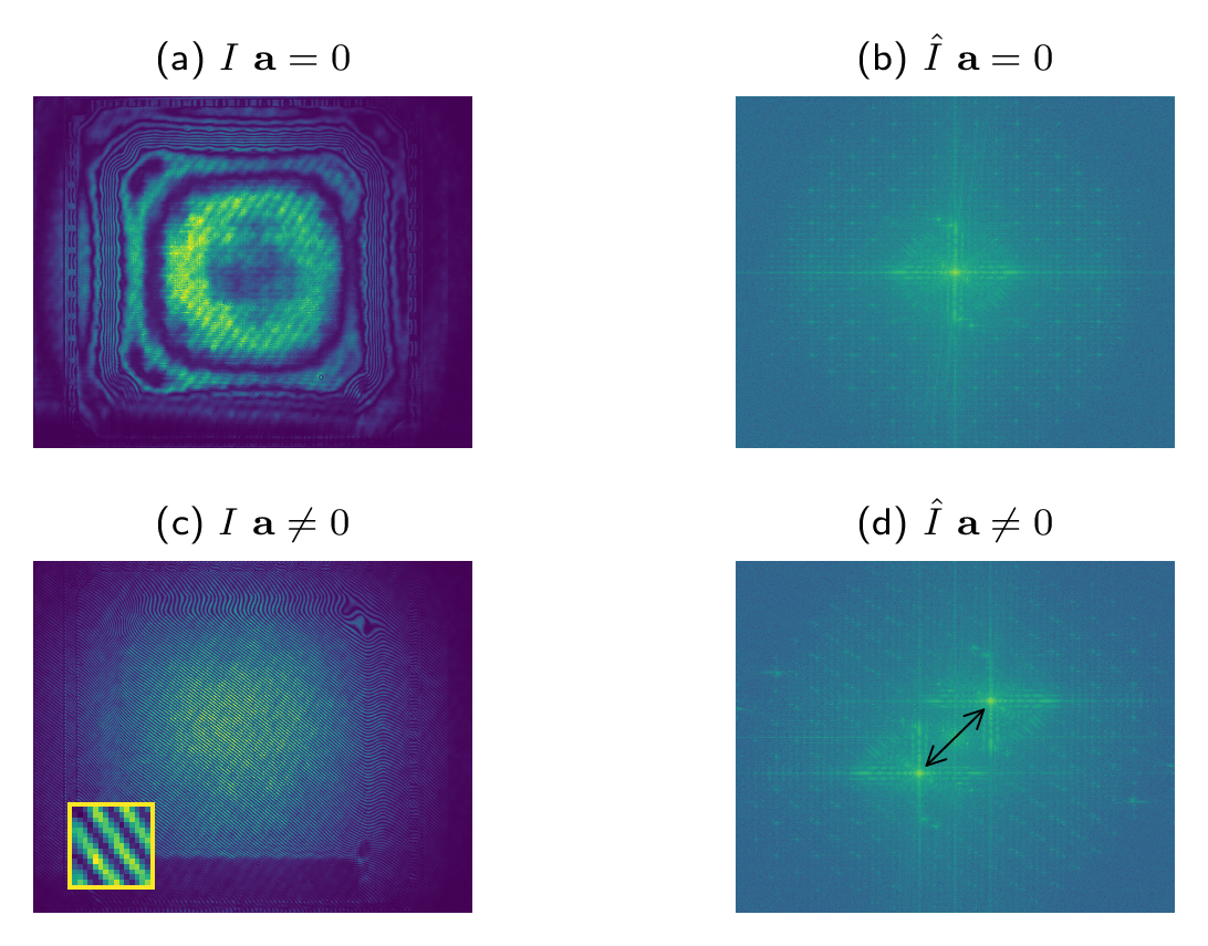
Figure 3 shows an interferogram and its Fourier transform when no tilt is present (\(\mathbf{a} = \mathbf{0}\); top row), and when a tilt is applied (bottom row). As \(\mathbf{a}\) increases in magnitude, the first-orders orders given by \(\mathcal{F}[ABe^{i\Phi}](\mathbf{y} \pm \mathbf{a})\) drift apart in the Fourier plane. This is highlighted by the double arrow within the plot in the bottom-right hand corner.
Figure 3: Retrieval of the test phase \(\Phi\) via frequency modulation.
(a) and (b) interferogram and its spectrum recorded when the tilt of
flat mirror FM is zero; (c) and (d) interferogram and its spectrum
recorded after applying a tilt; The inset in (c) shows
the frequency of the fringes in comparison to the pixel size.
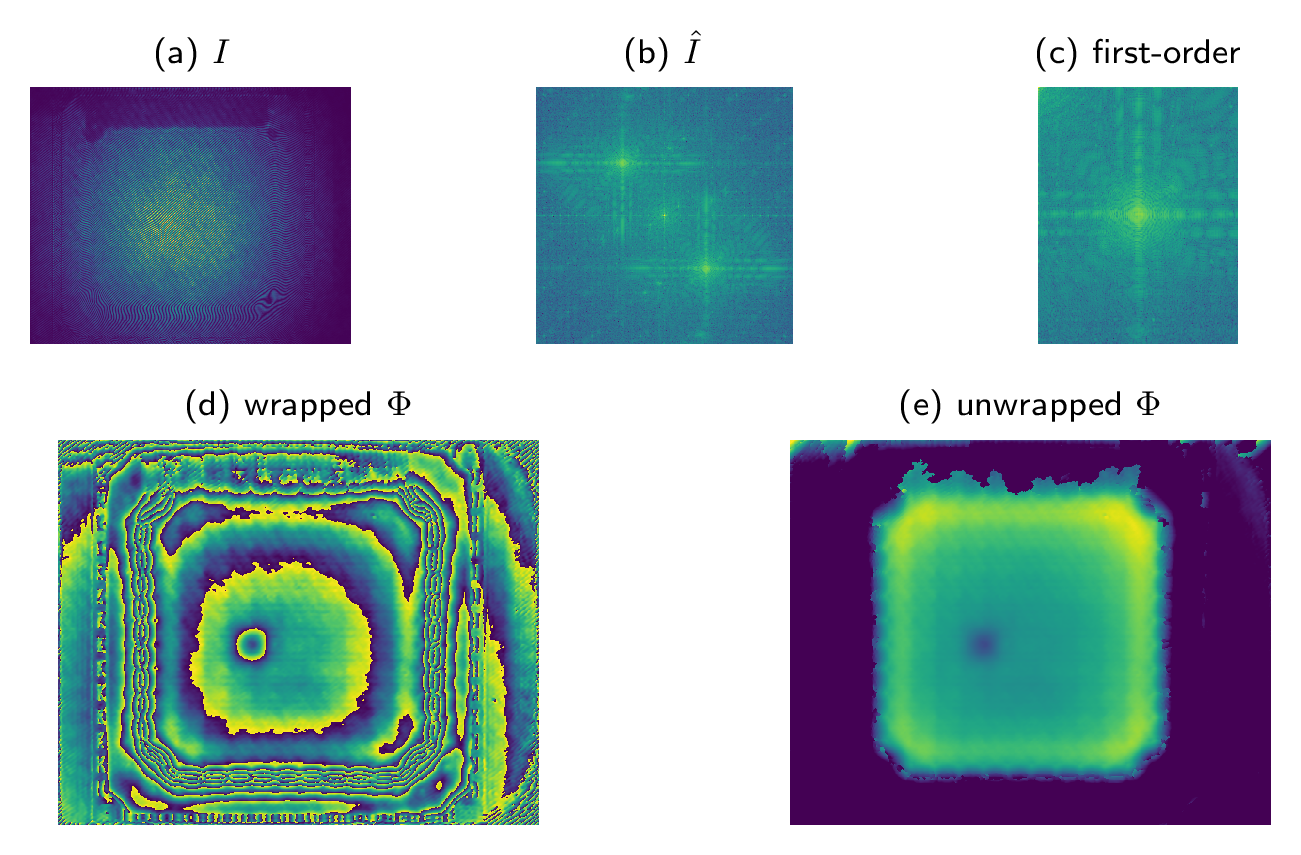
The steps necessary to obtain the test phase \(\Phi\) from the interferogram are outlined in Fig. 4. After computing the spectrum \(\hat{I}\), one of the first-orders \(\mathcal{F}[ABe^{i\Phi}](\mathbf{y} \pm \mathbf{a})\) is selected and translated back to the origin in the frequency space. Subsequently, one applies the inverse Fourier transform and extracts the phase by applying the \(\operatorname{arctan2}(\cdot)\) function, resulting in the wrapped phase shown in Fig. 4 (d). This latter phase can then be unwrapped to obtain the final estimate of \(\Phi\), as seen in Fig. 4 (e). Note that large tilts of FM make it easier to extract the first-orders and increase the resolution of the unwrapped phase. As a result it is preferable to apply tilt both in the \(x\) and \(y\) directions, so that the distance from the zero-order located at the origin in the frequency plane is maximised.
Figure 4: (a) original interferogram; (b) spectrum of the interferogram; (c)
first-order extracted from (b); (d) wrapped phase obtained by inverse
Fourier transforming (c); (e) phase after running the phase unwrapping
algorithm; In (e) one of the central actuators of the DM is pulled.
Using the method explained above one can sequentially poke each actuator of the DM and measure the corresponding influence function. In doing so one generates two sets of data which, for convenience, we collect into two matrices,
\[ \begin{equation} \begin{aligned} U &= \begin{bmatrix} \mathbf{u}_1, \dots, \mathbf{u}_D \end{bmatrix} \\ \Gamma &= \begin{bmatrix} \boldsymbol{\phi}_1, \dots, \boldsymbol{\phi}_D \end{bmatrix}. \end{aligned} \label{eq:Uphi} \end{equation}\]
Matrix \(\Gamma\) is particularly informative. In fact, one can apply the singular value decomposition (SVD) to obtain \(\Gamma = U_1 \Sigma_1 V_1^T\). Analysis of \(U_1\) and \(\Sigma_1\) reveals which shapes the DM can reproduce with high fidelity.
Calibration of the piston mode
As mentioned earlier, control of the piston mode is irrelevant for most microscopes, as this only affects the mean value of the phase and does not have any side effect on the quality of the recorded images. Nevertheless, this is not the case for 4Pi microscopes such as the one in . Here image formation relies on the interference of two foci created by two objectives arranged along a single optical axis and oriented in opposite directions. In this class of microscopes control of the piston mode is instead critical to ensure correct image formation. In this section we describe how one can adjust the arbitrary piston values found in \(\Gamma\) such that the calibration of the DM can also include the piston mode.
It should be remarked that the procedure described here is still significantly beneficial for conventional, non-4Pi microscopes as argued below. For conventional microscopes one could naively ignore the piston mode by arbitrarily setting the mean values of the columns of \(\Gamma\) to zero. Doing so, however, may lead to reduced or highly asymmetric stroke at a later stage when controlling the DM. For example, consider the case where a membrane DM is used and one wishes to apply spherical aberration. One may apply the actuation necessary to induce spherical aberration around the centre of the voltage range of the actuators or close to the maximum of the range. Clearly the former case is more desirable, as one can apply an approximately symmetric stroke of both positive and negative spherical aberration. In the latter case, instead, one easily incurs in saturation of the DM due to the proximity to the maximum of the voltage range. One can only ensure that this inconvenience is avoided by explicitly accounting for the piston mode in the calibration procedure.
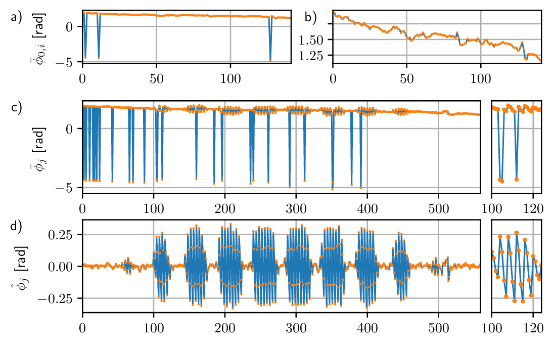
Calibration of the piston mode requires acquiring the output data \(\Gamma\) in a particular fashion. Below we describe in detail how we obtained \(\Gamma\) and which processing steps we applied. For clarity of exposition, we assume that the elements of \(\mathbf{u}\) are normalised such that they take values between -1 and 1. We then collected \(\Gamma\) by poking each actuator in \(2M + 1\) steps. In more detail, we chose matrix \(U\) above as \(U = I \otimes [-u_M, \ldots, 0, \ldots, u_M]\), where \(\otimes\) is the Kronecker product, \(I\) is the identity matrix, and \(u_M\) is the maximum actuation value. In doing so, we repeated the input \(\mathbf{u} = \mathbf{0}\) multiple times, and denoted the set of corresponding measurements by \(\{\boldsymbol{\phi}_{0, i}\}\), where \(i\) is the enumeration index. The remaining measurements where \(\mathbf{u} \neq \mathbf{0}\) were instead collected into another set denoted by \(\{\boldsymbol{\phi}_{j}\}\). The piston values \(\{\bar{\phi}_{0, i}\}\), computed as the mean values of \(\{\boldsymbol{\phi}_{0, i}\}\), are shown in Fig. 5 (a). Here it can be seen that some measurements are outliers with respect to the overall trend of the data, by multiples of \(2\pi\), which is a result of the arbitrary piston determined by the phase unwrapping algorithm applied to \(\boldsymbol{\phi}\). To correct for this, one-dimensional phase unwrapping was applied to \(\{\bar{\phi}_{0, i}\}\), along index \(i\), and the result is reported in Fig. 5 (b). This second graph shows the undesired effects of external disturbances to the measurements obtained from the interferometer. These variations were not due to displacement of the membrane of the DM, since the input was constant, i.e., \(\mathbf{u} = \mathbf{0}\). Note that here we are neglecting non-linear effects as mentioned earlier in the introduction.
The pistons \(\{\bar{\phi}_{j}\}\) of \(\{\boldsymbol{\phi}_{j}\}\) are plotted in Fig. 5 (c), where a subset of the measurements with indices between 100 and 124 is also shown in the smaller plot on the right for improved clarity. Measurements \(\{\boldsymbol{\phi}_{j}\}\) were affected by three different contributions. The first two were due to the phase offsets caused by the phase unwrapping and by the external disturbances to the interferometer, as in Fig. 5 (a). The third contribution, instead, was due to the effective optical path difference induced by movement of the membrane of the DM. Clearly, the first two contributions should be discarded to obtain an accurate calibration of the DM. This could be achieved by considering the interpolated values of \(\{\bar{\phi}_{0, i}\}\) from Fig. 5 (b) over the indices \(j\), resulting in a set \(\{\bar{\phi}_{0, j}\}\), where the relationship between the indices \(i\) and \(j\) is given by the sequence of input column vectors defined by matrix \(U\). At this point, for a fixed index \(j\) which we drop for clarity, one has that the piston \(\hat{\phi}\) solely due to the movement of the membrane was given by \(\hat{\phi} = \bar{\phi} + \bar{\phi}_{0} + 2k\pi\). Here integer \(k\) was due to the phase unwrapping of \(\boldsymbol{\phi}\), but could be estimated by rounding \((\bar{\phi} - \bar{\phi}_{0})/(2\pi)\). The resulting piston values \(\hat{\phi}\) are plotted in Fig. 5 (d), where one can identify the piston contributions due to poking each actuator monotonically from \(-u_M\) up to \(u_M\). This is more clearly apparent in the subset plot on the right. Note that the underlying assumption was that poking a single actuator of the DM did not induce a piston variation across the pupil that was in excess of a wavelength.
Figure 5: Overview of the data processing outlined in
Section 3.1 to calibrate the piston introduced by the
DM. (a) piston \(\bar{\phi}_{0, i}\) detected with the interferometer by
repeatedly measuring the DM membrane at rest, the abscissa corresponds to
index \(i\); (b) same as in (a), after applying one-dimensional phase
unwrapping along \(i\); (c) piston \(\bar{\phi}_{j}\) determined before the
adjustment described in Section 3.1, the abscissa
corresponds to index \(j\). A zoom of the graph between indices 100 and 124
is shown in the panel on the right; (d) piston \(\hat{\phi}\) determined after
applying the adjustment. A zoom of part of the graph is shown in the panel
on the right.
Modal control of the DM
After collecting the input–output measurements \(U\) and \(\Gamma\) one could compute matrix \(\Psi\) and its pseudo-inverse, which would allow control of the DM directly in terms of the phase grid \(\boldsymbol{\Phi}\) defined with Eq. \eqref{eq:Psiusamp}. This approach, however, is ill-suited to control or exclude certain DOFs, as outlined in the introduction. For example, a tilt due to the DM results in a corresponding shift of the current field of view (FOV), which is undesirable in scanning microscopes where positioning of the FOV is dealt with other hardware. Most importantly this also results in wasting some of the limited stroke of the DM, which is spent in translating the FOV instead of being available for aberration correction.
A more convenient strategy is to establish the control of the DM in terms of a modal basis such as Zernike polynomials [10; 11], which are a complete basis in the unit disk [12]. The first 28 Zernike polynomials are depicted in Fig. 6. When controlling the DM using Zernike polynomials one can ensure that no tilt is induced by the DM simply by setting to zero the coefficients with indices \(2\) and \(3\).
Figure 6: Table of the first 28 Zernike polynomials [11]. The
polynomials are normalised and enumerated according to a single index \(\#\)
defined by Noll [14]. The radial and azimuthal orders are
indicated by \(n\) and \(m\), respectively.

In analogy to Eq. \eqref{eq:Psiusamp}, one can express the phase \(\Phi\) induced by the DM as a linear combination of Zernike polynomials, i.e.,
\[ \begin{equation} \boldsymbol{\Phi} \approx Z \mathbf{z}. \label{eq:PhiZz} \end{equation}\]
Here \(Z\) is a matrix whose columns contain the Zernike polynomials sampled over the phase measurement grid, \(Z = [\bar{\mathbf{z}}_1, \ldots, \bar{\mathbf{z}}_{N_z}]\). The approximation sign in Eq. \eqref{eq:PhiZz} highlights that the validity of the equation is determined by the finite number of Zernike modes \(N_z\) considered. Note that the same equation applies also in case other modal decompositions are employed. Furthermore, in this tutorial we assume \(N_z > N_a\). This assumption is justified by the fact that the influence functions of the DM do not resemble Zernike polynomials. As a result, more Zernike polynomials are necessary to describe the influence functions without encountering large approximation errors.
Computation of \(H\) from experimental data
In the next step we assume that there exists a matrix \(H\) of dimensions \(N_z \times N_a\), which describes the linear mapping between the input control signal \(\mathbf{u}\) applied to the DM and the output Zernike coefficients \(\mathbf{z}\),
\[ \begin{equation} \mathbf{z} \approx H \mathbf{u}. \label{zHu} \end{equation}\]
Matrix \(H\) can be estimated from the experimental data \(\Gamma\) and \(U\), by minimising the following cost function
\[ \begin{equation} \underset{H}{\operatorname{min}} \; \sum_{i=1}^{D} \| \boldsymbol{\Phi}_i - ZH\mathbf{u}_i \|^2, \label{eq:minH} \end{equation}\]
which expresses the total error in predicting the measured output phases \(\boldsymbol{\Phi}\) by means of \(H\). After some linear algebra manipulations, it can be shown that the optimal \(H\) that minimises Eq. \eqref{eq:minH} satisfies the following normal equation [15]
\[ \begin{equation} Z^TZH \left( \sum_{i=1}^{D} \mathbf{u}_i \mathbf{u}_i^T \right) = Z^T \left( \sum_{i=1}^{D} \boldsymbol{\Phi}_i\mathbf{u}_i^T \right), \label{eq:normaleq} \end{equation}\]
which allows us to compute \(H\).
To build some intuition behind Eq. \eqref{eq:normaleq}, we can consider the simpler case where \(U = I_{N_a}\), which corresponds to poking each actuator once only with unit amplitude. As a result, we collect one measurement for each of the influence functions of the DM, i.e., \(\Gamma = [\boldsymbol{\psi}_1, \ldots, \boldsymbol{\psi}_{N_a}]\). Furthermore, we can observe that \(Z^TZ\) is approximately proportional to the identity matrix \(I_{N_z}\), due to the orthogonality property of Zernike polynomials. Since \(\sum_{i=1}^{D} \mathbf{u}_i \mathbf{u}_i^T = I_{N_a}\), we have that
\[ \begin{equation} \begin{aligned} H \approx Z^T \left( \boldsymbol{\psi}_1\mathbf{e}_1^T + \ldots + \boldsymbol{\psi}_{N_a}\mathbf{e}_{N_a}^T \right) &= [\bar{\mathbf{z}}_1, \ldots, \bar{\mathbf{z}}_{N_z}]^T \cdot [\boldsymbol{\psi}_1, \ldots, \boldsymbol{\psi}_{N_a}] \\ &= Z^T \Gamma, \end{aligned} \end{equation} \label{eq:normaleqexp}\]
where \(\mathbf{e}\) are the unit vectors from the standard basis. Here we can see that the columns of matrix \(H\) are equal to the inner products of the sampled Zernike polynomials with the influence functions of the DM. For example, the first column of \(H\) is given by
\[ \begin{equation} \mathbf{h}_1 \approx \begin{bmatrix} \bar{\mathbf{z}}_1^T \boldsymbol{\psi}_1 \\ \vdots \\ \bar{\mathbf{z}}_{N_z}^T \boldsymbol{\psi}_1 \label{eq:single} \end{bmatrix}. \end{equation}\]
Therefore the substantial difference between using Eq. \eqref{eq:single} and Eq. \eqref{eq:normaleq} to estimate \(H\) is that with Eq. \eqref{eq:normaleq} one estimates \(H\) using a single linear regression that minimises Eq. \eqref{eq:minH}, which is more robust to measurement noise in general.
Computation of the control matrix \(C\)
Once matrix \(H\) is known, it can be used to control the DM using the selected basis functions. In more detail, given a desired shape of the DM expressed via the vector of modal coefficients \(\mathbf{z}\), one seeks to find the input \(\mathbf{u}\) that minimises the following cost function,
\[ \begin{equation} \underset{\mathbf{u}}{\operatorname{min}} \; \| \mathbf{z} - H\mathbf{u} \|^2, \end{equation}\]
which is solved in a least-squares sense by letting \(\mathbf{u}=H^\dagger \mathbf{c}\), where \(H^\dagger\) is the pseudo-inverse of \(H\). Matrix \(H^\dagger\) is commonly referred to as the control matrix \(C\) in AO literature [16]. In particular, one can implement a simple proportional controller by letting \(\mathbf{u} = C \mathbf{z}\), where the measurement of \(\mathbf{z}\) is provided by a wavefront sensor. In sensorless adaptive optics [3], instead, operation of the DM is performed in open-loop, and the relationship \(\mathbf{u} = C \mathbf{z}\) is just assumed to hold.
It is important to recall that matrices \(H\) and \(C\) are relevant for a particular arrangement of the pupil with respect to the active area of the DM. This means that one should recompute these matrices to account for any change in the reimaging of the BFP onto the DM. Examples of such changes are stopping down the pupil with an aperture, or shifting the position of the DM.
Regularisation approaches
It is often the case that one encounters difficulties when computing \(C\) naively as described above. For example, consider the phase shown in the top-left hand corner of Fig. 1. It is clear that poking the corresponding actuator induces a negligible phase contribution within the selected pupil. In linear algebra terms this phenomenon is revealed as a negligible singular value \(s_{N_a}\) within the SVD of \(H\). This is given by \(H= U_2 \Sigma_2 V_2^T\), where
\[ \begin{equation} \Sigma_2 = \begin{bmatrix} s_1 & &\\ & \ddots & \\ & & s_{N_a} \\ & \mathbf{0} & \end{bmatrix}, \end{equation}\]
and \(s_1 \gg s_{N_a}\). As a result, depending on the value of \(\mathbf{z}\), the control values computed by evaluating \(\mathbf{u} = C \mathbf{z}\) may result in unreasonably large values. To obviate this issues one can resort to regularisation methods. Among many possible options, one can opt for Tikhonov regularisation [17].
Design of a compact slot-in interferometer
In this section we describe in detail how to build a compact, slot-in interferometer using off-the-shelf optomechanical components. One can temporarily insert this interferometer into an existing microscope setup that comprises DMs but has no permanent interferometer in place. The slot-in interferometer can then be used for DM calibration and troubleshooting.
Optomechanical design
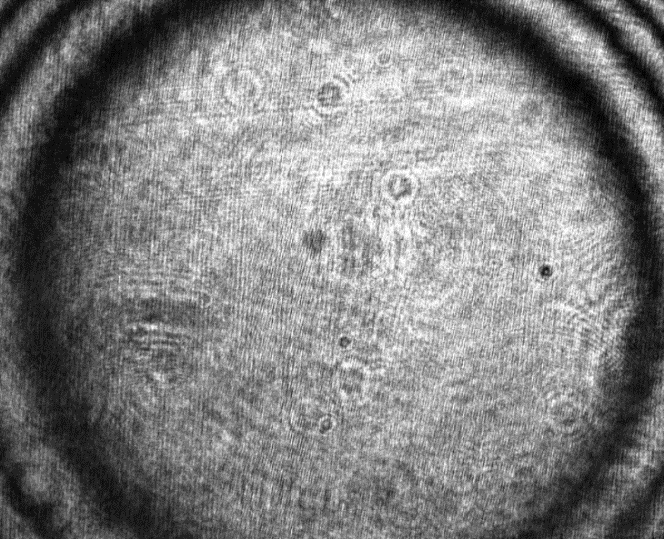
The layout and technical drawing of the compact interferometer are shown in Fig. 7 and Fig. 8, respectively. The list of parts is reported in Tab. 1. A picture of the assembled interferometer is shown in Fig. 9. Note that a single conjugation between the DM and the camera is present in Fig. 7, in contrast with Fig. 2. This compromise has been selected to enhance the compactness of the design. During assembly of the interferometer, one should pay attention to the alignment and conjugation of the 4f system comprising lens L1 and L2. One option is to check the correct collimation with a shearing interferometer. A flat mirror can also be used as a target to test the interferometer, as seen in Fig. 10. Here it can be seen that some field curvature is present, which is a result of the compact design of the interferometer. Nevertheless, this has negligible effect on the DM calibration if the active area of the DM is well inscribed within the central disk. Additionally, one can measure the phase errors due to the non-flatness of the field with a flat mirror and subsequently subtract these from the phase measurements obtained with the DM, thus resulting in corrected measurements of the phase.
Figure 7: Layout of the compact slot-in interferometer. A wedge prism (WP)
is used instead of a flat mirror to reduce the necessary angular offset
between the reference and test arms of the interferometer.

Figure 8: Technical drawing of the compact slot-in interferometer.

Figure 9: Picture of the assembled compact interferometer, which
is mounted in front of a flat mirror visible in the top-right.
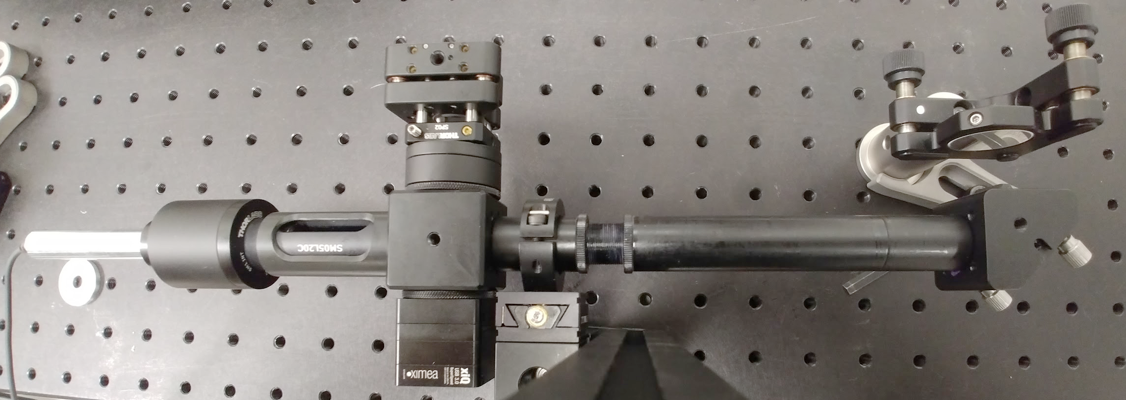
Figure 10: Interferogram obtained with the slot-in interferometer when
measuring a flat mirror. Note that even though some field curvature is
visible, this has negligible effect for the DM calibration, provided the
active area of the DM is well inscribed in the central disk. This
compromise was intentional, in order to maximise the compactness of the
design of the interferometer.
| Item | Qty | Part number | Maker | Description |
|---|---|---|---|---|
| 1 | 1 | CCM5-BS016/M | Thorlabs | Mounted beamsplitter |
| 2 | 1 | KCB05/M | Thorlabs | Right-angle kinematic mirror mount |
| 3 | 1 | KC05-T/M | Thorlabs | 0.5" kinematic mount |
| 4 | 2 | SM1A1 | Thorlabs | Ext SM05 to int SM1 |
| 5 | 1 | SM1L05 | Thorlabs | 0.5" long SM1 |
| 6 | 1 | PS810-A | Thorlabs | Wedge prism |
| 7 | 1 | SM1W353 | Thorlabs | Wedge prism mount ring |
| 8 | 1 | SP02 | Thorlabs | SM05 cage plate |
| 9 | 1 | SM05L20C | Thorlabs | Slotted SM05, 2" |
| 10 | 1 | MQ013MG-ON | Ximea | Camera |
| 11 | 1 | SM05A1 | Thorlabs | Ext C-mount to ext SM05 |
| 12 | 1 | XE25L225/M | Thorlabs | 225 mm Long Construction Rail |
| 13 | 1 | CPS532 | Thorlabs | 532nm diode laser |
| 14 | 1 | AD11F | Thorlabs | Diode laser mount |
| 15 | 1 | CPS1 | Thorlabs | 5V diode laser power supply |
| 16 | 2 | PF05-03-P01 | Thorlabs | 0.5" protected silver mirror |
| 18 | 4 | SR1.5 | Thorlabs | 1.5" cage rod |
| 19 | 1 | DT12/M | Thorlabs | 5mm travel stage |
| 20 | 1 | RM1G | Thorlabs | 1" construction cube |
| 21 | 1 | SM05A3 | Thorlabs | Ext SM05 to ext SM1 |
| 22 | 1 | SM05L30 | Thorlabs | 3" SM05 |
| 23 | 1 | SM05T10 | Thorlabs | SM05 coupler |
| 24 | 2 | SM05L10 | Thorlabs | 1" SM05 |
| 25 | 1 | SM05TC | Thorlabs | SM05 clamp |
| 26 | 2 | 47-668 | Edmund | F=60mm achromat, 12.5mm dia |
| 27 | 1 | LA1213-A | Thorlabs | F=50mm plano-convex, 0.5" dia |
| 28 | 1 | LC2632-A | Thorlabs | F=-12mm plano-concave, 6mm dia |
| 29 | 1 | LMRA6 | Thorlabs | LMR/SM05 adapter for 6mm optics |
Table 1: Parts list for the compact interferometer.
Additional notes
Note that laser diodes have shorter coherence lengths than other sources such as HeNe lasers for example. Therefore, one has more stringent demands in terms of matching the optical path lengths of the two arms in Fig. 7. The choice of a diode laser was made in order to maximise the compactness of the design and minimise cost. If the contrast of the fringes is too low when using a diode laser, it may be helpful to shut down the laser for a short period, e.g. a minute. Alternatively one may consider replacing the diode laser with a fibre coupled laser source exhibiting longer coherence length.
Threadlock, e.g. Loctite 222 Purple Pipe & Thread Sealant Liquid can be used to align the camera and lock it with item 23. Item DT12/M should also be locked to avoid susceptibility to vibrations.
DM calibration toolbox
A toolbox for DM calibration written in Python is freely available at the following address.
This toolbox supports a number of DMs and scientific cameras from different manufacturers. With this hardware, the toolbox can be immediately used to calibrate a DM. The toolbox also includes two GUIs – one for the DM calibration and the other for control of the DM using Zernike modes. If the user application is written in Python using the PyQt toolkit, one can embed the GUIs directly into the host application. Alternatively, if the DM and camera hardware are not directly supported, one can use the toolkit as an external library, driving the hardware using their own software. The result of the calibration is saved into an HDF5 file, which can be loaded from third-party software.
Conclusions
In this tutorial we discussed how to perform the calibration of a deformable mirror (DM) using an interferometer. The interferometer can be built into the microscope and used for calibration and subsequent troubleshooting of the DM. Alternatively, we presented the design of a compact, slot-in interferometer, which can be temporarily inserted into an existing microscope to perform the DM calibration. Finally, we provide a toolbox written in Python to perform the DM calibration, which can be downloaded for free.
References
[1] J. A. Kubby, ed., Adaptive Optics for Biological Imaging (CRC press, 2013).
[2] G. Vdovin, O. Soloviev, M. Loktev, and V. Patlan, OKO Guide to Adaptive Optics (Flexible Optical B.V., 2013), 4th ed.
[3] M. J. Booth, "Adaptive optical microscopy: the ongoing quest for a perfect image," Light Sci. Appl. 3, e165 (2014).
[4] M. Booth, T. Wilson, H.-B. Sun, T. Ota, and S. Kawata, "Methods for the characterization of deformable membrane mirrors," Appl. Opt. 44, 5131-5139 (2005).
[5] D. Débare, T. Vieille, and E. Beaurepaire, "Simple characterisation of a deformable mirror inside a high numerical aperture microscope using phase diversit," J. Microsc 244, 136-143 (2011).
[6] D. Malacara, Optical shop testing, (John Wiley & Sons, 2007).
[7] M. Peck, "Interferometry mathematics, algorithms, and data,". Accessed: 03 Feb 2016.
[8] M. Takeda, H. Ina, and S. Kobayashi, "Fourier-transform method of fringe-pattern analysis for computer-based topography and interferometry," J. Opt. Soc. Am. 72, 156-160 (1982).
[9] T. I. M. van Werkhoven, J. Antonello, H. H. Truong, M. Verhaegen, H. C. Gerritsen, and C. U. Keller, "Snapshot coherence-gated direct wavefront sensing for multi-photon microscopy," Opt. Express 22, 9715-9733 (2014).
[10] F. Huang, G. Sirinakis, E. Allgeyer, L. Schroeder, W. Duim, E. Kromann, T. Phan, F. Rivera-Molina, J. Myers, I. Irnov, M. Lessard, Y. Zhang, M. Handel, C. Jacobs-Wagner, C. Lusk, J. Rothman, D. Toomre, M. Booth, and J. Bewersdorf, "Ultra-high resolution 3D imaging of whole cells," Cell 166, 1028-1040 (2016).
[11] F. Zernike, "Beugungstheorie des Schneidenverfahrens und seiner verbesserten Form, der Phasenkontrastmethode," Physica 1, 689-704 (1934).
[12] V. N. Mahajan, "Zernike circle polynomials and optical aberrations of systems with circular pupils," Appl. Opt. 33, 8121-8124 (1994).
[13] M. Born and E. Wolf, Principles of Optics (Cambridge University Press, 1999), 7th ed.
[14] R. J. Noll, "Zernike polynomials and atmospheric turbulence," J. Opt. Soc. Am. 66, 207-211 (1976).
[15] J. Antonello, T. van Werkhoven, M. Verhaegen, H. H. Truong, C. U. Keller, and H. C. Gerritsen, "Optimization-based wavefront sensorless adaptive optics for multiphoton microscopy," J. Opt. Soc. Am. A 31, 1337-1347 (2014).
[16] C. Paterson, I. Munro, and J. Dainty, "A low cost adaptive optics system using a membrane mirror," Opt. Express 6, 175-185 (2000).
[17] P. C. Hansen, Discrete Inverse Problems (Society for Industrial and Applied Mathematics, 2010).
Return to documents