Calibration and Closed-Loop Control of Deformable Mirrors Using Direct Sensing

1. Introduction

When implementing an adaptive optics (AO) system in a microscope, there are a number of factors to consider. For example, the choice of wavefront corrector and whether or not to use a wavefront sensor. In all cases, calibration of the correction device is necessary. The purpose of this tutorial is to outline the steps involved in implementing deformable mirror calibration and control in closed-loop using direct wavefront sensing with the Shack-Hartmann sensor. The advantages of this approach will also be discussed. Note that a deformable mirror and a Shack-Hartmann sensor are used in this tutorial, as these are the most widely used components in the AO literature. However, the concepts presented here could be applied to other types of correctors and sensors.

2. Why use a Closed-Loop System?

The main difference between a closed-loop and open-loop system is the arrangement of the AO components with respect to each other. This difference is shown in Figure 1 for a simple confocal fluorescence imaging system. In a closed-loop system, as shown in Figure 1(a), the light returning from the sample passes via the deformable mirror before it reaches the sensor. This means that the sensor measures the error in the aberration correction, rather than the full induced aberration. In effect, the sensor provides feedback on whether the deformable mirror has reached the desired shape to obtain an aberration-free, i.e. plane, wavefront. In an open-loop system, as shown in Figure 1(b), there is no feedback on whether the deformable mirror has acquired the correct shape, as the light does not pass via the deformable mirror when returning from the sample. The advantage of using a closed-loop system is that it can be more accurate; any non-linearities in the movement of the mirror surface with applied voltage are inherently compensated, as are hysteresis and drifts in the shape of the mirror are corrected for. Note that in the diagrams there is an aperture conjugate to the sample plane. This assists with preventing light scattered from multiple depths affecting the sensor measurements. This aperture must be larger than the usual confocal pinhole so that the aberration information is not filtered out.

There are three important points to note from the diagrams. The first is that the deformable mirror (and sensor) are in a pupil conjugate plane, as this is usually the way AO is implemented. However, a small number of studies have shown that placing the corrector conjugate to the sample has the potential to correct for aberrations over a wider field-of-view, see for example [1]. The second point to note is that the light returning from the sensor passes via the deformable mirror before reaching the imaging device. This is because in a confocal system the final point spread function (PSF), and so resolution, is affected by the ingoing and outgoing PSF. In a two-photon system, this is not the case. The resolution depends on being able to form a tight focus in the sample. Consequently, the photodetector need not be after the corrector and would be placed close to the sample where it acts as a 'bucket' to collect as much returning light as possible. The third point is that the Shack-Hartmann sensor is placed in a de-scanned path, meaning that the light returning from the sample does not pivot on the lenslet array and each microlens focus is stationary during the scan. This is because traditional algorithms for analysing Shack-Hartmann images rely on a single focus forming behind each microlens on the Shack-Hartmann camera. However, this need not necessarily be the case [2].

3. Wavefront Sensing

Although sensorless control schemes require less hardware, one of the main advantages of direct sensing is speed. All aberrations can be simultaneously measured and corrected using a single measurement. Although there are many devices that can be used to measure aberrations, the most common device used in AO is the Shack-Hartmann sensor as it is simple and effective. The principle of the Shack-Hartmann sensor is shown in Figure 2. The pupil of the objective is imaged onto an array of microlenses as shown in Figure 2(a). When there are no aberrations, the wavefront is plane. This results in a regular array of spots being formed on a camera placed at the focal length of the lenslet array. When the wavefront is aberrated, the spots will shift their location according to the tilt of the wavefront across each lenslet as shown in Figure 2(b). The slope of the wavefront in the \(y\)-direction, \(S_y\) for each lenslet is given by:

\[ S_{y} = \frac{{\mathrm{\Delta}W}_{y}}{a} = \frac{y - y_{0}}{f} = \frac{\mathrm{\Delta}y}{f} \tag{1}\]

where \({\mathrm{\Delta}W}_{y}\) is the wavefront tilt, a is the diameter of a lenslet, \(y_0\) is the location of the spot when no aberrations are present, \(y\) is the location for an aberrated wavefront, and \(f\) is the focal length of the lenslet array. A similar expression exists for \(x\). Note that in Figure 2, the lenslets have flat edges at the top and bottom. This is so that the lenslets are contiguous with no light lost in the gaps between them. Care must be taken when choosing a lenslet array to ensure that this is the case, if optical efficiency is important.

3.1 Selecting the Lenslet Array

When choosing the lenslet array there are two main factors to consider:

1) The number of lenslets sampling the pupil.

2) The focal length of the lenslet array.

The number of lenslets sampling the pupil depends upon the pitch of the lenslet array (the pitch is equivalent to the lenslet diameter for a fully filled array) and the magnification between the objective aperture and the lenslet array. The higher the number of lenslets sampling the pupil, the higher is the spatial resolution of the measurements. However, this will lead to a lower signal to noise ratio for each spot as there will be less light per lenslet. A value of 2 for the ratio of total number of lenslets to total number of actuators has been found to be sufficient for vision science adaptive optics systems, however in astronomical adaptive optics systems, a lower value has been used [3, 4].

When selecting the focal length, there is a trade-off between dynamic range and sensitivity as shown in Figure 3. Dynamic range can be defined as the maximum measurable tilt across a lenslet before the spot crosses into the region behind a neighbouring lenslet. This is the tilt corresponding to a shift in the spot of \(a/2\). Hence the maximum measurable tilt is:

\[ {\mathrm{\Delta}W}_{\text{Max}} = \frac{a^{2}}{2f} \tag{2}\]

Therefore, the longer the focal length, the smaller the dynamic range. However, the shorter the focal length, the less sensitive the Shack-Hartmann is to the tilt across each lenslet. The minimum measurable tilt is given by:

\[ {\mathrm{\Delta}W}_{\text{Min}} = \frac{{\mathrm{\Delta}y}_{\text{Min}}a}{f} \tag{3}\]

where \({\mathrm{\Delta}y}_{\text{Min}}\) is the minimum measureable spot displacement which depends on factors such as the noise level. In practice, the focal length should be chosen based on the stroke of the mirror (or the actual stroke one will be using). The focal length should be such that full deflection of the surface of one actuator, from its mid-stroke position, does not cause a spot to move in to the region behind a neighbouring lenslet. Note from Equations 2 and 3 that the sensitivity and dynamic range are also affected by the diameter of each lenslet. However, it is assumed that this value is set when determining the number of lenslets per actuator.

3.2 Selecting the Camera

A wide range of CMOS and CCD cameras has been used in Shack-Hartmann sensors. Factors to consider are the quantum efficiency and noise level. Improvements in such performance factors must be balanced with the cost. Note that when using the Shack-Hartmann sensor to merely calibrate a deformable mirror, with a view to implement sensorless AO for example, the camera does not need to be very sensitive as laser light can directly be used directly. However, when using the Shack-Hartmann sensor to perform closed-loop correction of sample aberrations using fluorescence emission, the light intensity returning from the sample will likely be low and a more sensitive camera will be required.

3.3 Determining Spot Location

The location of the spot behind each lenslet is typically determined using a centre-of-mass algorithm; this process is referred to as centroiding. The \(x\) and \(y\) locations, i.e. centroids of a spot, (\(C_x\),\(C_y\)), are given by:

\[ C_x=\frac{\sum_{i=1}^N{x_il_i}}{\sum_{i=1}^N{I_i}}, C_y=\frac{\sum_{i=1}^N{y_il_i}}{\sum_{i=1}^N{I_i}} \tag{4}\]

where \(x_i\) and \(y_i\) are the coordinates of the \(i^{th}\) pixel, \(I_i\) is the intensity of the \(i^{th}\) pixel and N is the total number of pixels. The assignment of the pixel coordinates and pixel numbers are as shown in Figure 4 for a simplified example of a sensor where there are nine camera pixels behind a single lenslet. When there are no aberrations, the spot has coordinates of (0,0) as shown in Figure 4(a). When aberrations are present the spot has moved to (0.25,-0.25) as shown in Figure 4(b).

4. Calibration

The aim of the calibration procedure is to determine the relationship between the sensor signals and the control signals sent to the deformable mirror. Once this is determined, the required control signals to correct a given set of sensor measurements can readily be calculated. An effective way to perform this calibration is to use a fluorescent bead as the sample. Note that a mirror in place of the sample should not be used. The reason for this is illustrated in Figure 5. During the calibration process, the light will pass via the deformable mirror twice: once on the way to the sample and once from the light returning from the sample. If a mirror is used then the light reflected will retain the phase information from the first pass as shown in Figure 5(a). Consequently, the wavefront the Shack-Hartmann sees is not a true representation of the shape of the deformable mirror. This is akin to the well-known double pass effect whereby odd symmetry aberrations cancel out between the two paths and even symmetry aberrations are doubled in amplitude. These problems are avoided when using a fluorescent object. As fluorescence is an incoherent process, the phase information on the first pass is lost and only the phase information from the emission path is retained, giving a true representation of the effect of the deformable mirror, as shown in Figure 5(b).

4.1 Obtaining the Matrix Influence Functions

When a control signal is applied to a given actuator, the surface attains a characteristic shape referred to as the influence function. The shape of the mirror surface can be considered to be the sum of these functions (assuming it operates in a linear manner, which is usually a good approximation). Consequently, measurement of the influence functions characterises the properties of the mirror.

Note that for an electrostatically actuated device, the deflection of the mirror surface is proportional to the square of the applied voltage. Consequently, in order to drive the device in a linear fashion, the normalised control signal would be given by \({(V/V_{\max})}^{2}\), where \(V_{\max}\) is the maximum voltage that can be applied and 0 is the minimum. For electromagnetically actuated devices, the displacement is proportional to the applied current, which can be positive or negative, producing displacements in both directions. The control signal is therefore defined to be proportional to the current.

The calibration procedure is shown in Figure 6. Before measuring these influence functions, the mirror is set to its mid-stroke position. This is because that when the mirror corrects for a given wavefront, the mirror needs to be able to move forwards and backwards depending on which parts of the wavefront are advanced and which parts are delayed. For an electromagnetically-actuated device, for example, the surface is at the mid-stroke position when half of the control signal range is applied to each actuator. This corresponds to zero as the device is driven using positive and negative values. For an electrostatically-actuated device, \(\sqrt{0.5}V_{\max}\) is applied to each actuator to obtain the mid position. During the calibration procedure, the control signal for each actuator is increased then decreased, relative to the mid-stroke control signal. Note in the example shown in Figure 6 that increasing the control signal results in the surface moving upwards relative to its mid-point position. This depends upon the device however. Then the change in slopes per unit control signal or Zernike aberration coefficients per unit control signal are calculated. The influence function for each actuator forms a column in the so-called Influence Functions Matrix. Each element of the influence functions matrix, \(\text{IFS}\), for the slopes representation is given by:

\[ \text{IFS}_{l,Actuator} = \frac{S_{\text{lx}}^{+ C} - S_{\text{lx}}^{- C}}{2C} \tag{5}\]

\[ \text{IFS}_{l + NoLenslets,Actuator} = \frac{S_{\text{ly}}^{+ C} - S_{\text{ly}}^{- C}}{2C} \tag{6}\]

where \(l\) is the lenset number, \(\text{Actuator}\) is the actuator number, and \(S_{\text{lx}}^{+ C}\)and \(S_{\text{lx}}^{- C}\) are the slopes in the \(x\)-direction for lenslet \(l\) when a positive or negative control signal, \(C,\) is applied relative to the mid-stroke control signal, respectively; similarly, for \(y\). When using Zernike aberration coefficients:

\[ \text{IFZ}_{coeff,Actuator} = \frac{a_{\text{coeff}}^{+ C} - a_{\text{coeff}}^{- C}}{2C} \tag{7}\]

where \(a_{\text{coeff}}^{+ C}\) and \(a_{\text{coeff}}^{- C}\) are the Zernike aberration coefficients for coefficient number \(\text{coeff}\) when a positive or negative control signal, \(C,\) is applied relative to the mid-stroke control signal, respectively.

The conversion of slopes to Zernike aberration coefficients can be found using:

\[ \mathbf{a} = \mathbf{Z}^{\mathbf{+}}\mathbf{S} \tag{8}\]

where \(\mathbf{a}\) is a vector of Zernike coefficients, \(\mathbf{Z}^{\mathbf{+}}\) is the pseudo-inverse matrix of the Zernike slopes matrix \(\mathbf{Z}\), and \(\mathbf{S}\) are the wavefront slopes:

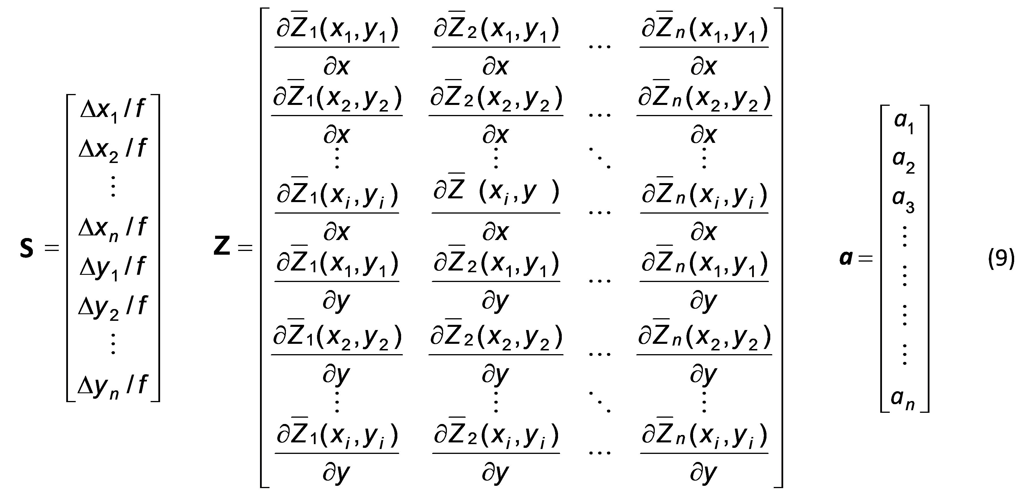
where \(f\) is the focal length of the lenslet array. The coordinates \((x_i,y_i)\) are the coordinates of each lenset. Note that as the Zernike polynomials are only orthogonal over a unit circle, the coordinates must be normalised. Although continuous Zernike polynomials are orthogonal, they may not necessarily be so when evaluated at discrete points, as in the case here. Consequently, Gram-Schmidt orthogonalisation, or another method, may be necessary. When determining the number of Zernike aberrations to reconstruct the slopes, care must be taken to ensure that the number of Zernikes used does not exceed the number of lenslets, otherwise the system would be underdetermined [5].

4.2 Obtaining the Control Matrix

Once the influence functions matrix has been determined, the required control signals, \(\mathbf{C},\) are given by:

\[ \mathbf{C} = \mathbf{(IFS}^{\mathbf{+}}\mathbf{)S} \tag{10}\]

where \(\mathbf{\text{IFS}}^{\mathbf{+}}\) is the pseudo-inverse of the influence functions matrix in term of slopes and S is a vector of measured slopes. Similarly, when the influence functions matrix is in terms of Zernike polynomial coefficients:

\[ \mathbf{C} = \mathbf{(IFZ}^{\mathbf{+}}\mathbf{)a} \tag{11}\]

where \(\mathbf{\text{IFZ}}^{\mathbf{+}}\) is the pseudo-inverse of the influence functions matrix in term of Zernike aberration coefficients and a are the coefficients. \(\mathbf{\text{IFS}}^{\mathbf{+}}\)and \(\mathbf{\text{IFZ}}^{\mathbf{+}}\)are referred to as the control matrices.

The pseudo-inverse is obtained using a technique called singular value decomposition (SVD). Just as the wavefront can be considered to consist of a sum of independent Zernike polynomials, the correction capability of the system can be considered to consist of the sum of independent system modes. These modes result from the SVD of the influence functions matrix and are equal in number to the number of actuators. SVD decomposes the influence functions matrix, \(\mathbf{\text{IF}}\), into three separate matrices, as shown in Figure 7(a):

\[ \mathbf{\text{IF}} = \mathbf{\text{US}}\mathbf{V}^{\mathbf{T}} \tag{12}\]

where the rows of \(\mathbf{V}^{\mathbf{T}}\) represents each mode in actuator space, i.e. the control signals applied to each actuator to generate a given surface shape. These can be thought of as mirror modes. When correcting a given wavefront, the mirror will use a combination of these independent mirror modes to perform the correction. The columns of \(\mathbf{U}\) represent the modes as seen by the sensor, i.e. the sensor measurements that correspond to a mode driven by the mirror. If the influence functions matrix is in terms of slopes, each column vector will be a column vector of slopes; or, each column vector will be a vector of Zernike coefficients. The so-called singular values in the matrix \(\mathbf{S}\) link the modes together. For example, when a mirror mode is generated, the mode in sensor space is the singular value multiplied by the sensor space representation. They singular values are ordered from their lowest to highest. Failure to use the singular values matrix correctly can make or break the performance of your AO system.

The pseudo-inverse, \(\mathbf{I}\mathbf{F}^{\mathbf{+}},\mathbf{\ }\)as illustrated in Figure 7(b), is given by:

\[ \mathbf{I}\mathbf{F}^{\mathbf{+}} = \mathbf{\text{V}}\mathbf{S}^{\mathbf{- 1}}\mathbf{U}^{\mathbf{T}} \tag{13}\]

From Equation 13 it is evident that when calculating the pseudo-inverse, the singular values are inverted. These become the mode gains. Small singular values result in high gains. This means that in order to produce the corresponding mirror mode, large control signals are required which will saturate the actuator control signals, i.e. the control signals will reach or exceed their maximum value. To remove these modes from the final calculation of the control matrix, the corresponding gains are set to zero. While this a common method, it is important to note that there are variations on this [7].

Figure 8(a) shows an example of four mirror modes when measuring the influence functions of the central 64 actuators of a Boston Micromachines 140 actuator deformable mirror with 177 lenslets. Figure 8(b) plots the singular values and gains (inverse of the singular values). These values have been normalised for display purposes. It can be seen that after around 55 modes there is a sharp rise in the gain. Hence removing modes 56 to 60 would be advisable. Note that the singular values are specific to a given set-up, i.e. the number of actuators and number of lenslets, and their alignment relative to each other. Too large a decrease in the number of modes used can result in reduced fidelity of the correction.

5. Implementing the Control Signals

When correcting the aberrations in a closed-loop system, the control signals can be implemented using:

\[ \mathbf{C}_{\mathbf{\text{New}}} = \mathbf{C}_{\mathbf{\text{Current}}} + {g\mathbf{(IFS}}^{\mathbf{+}})\mathbf{S}_{\mathbf{\text{Meas}}} \tag{14}\]

where \(\mathbf{C}_{\mathbf{\text{New}}}\mathbf{\ }\)are the new control signals, \(\mathbf{C}_{\mathbf{\text{Current}}}\) are the current control signals, \(g\) is the gain ( a value between zero and one to limit oscillations in the mirror surface), \(\mathbf{\text{IFS}}^{\mathbf{+}}\mathbf{\ }\)is the control matrix (pseudo-inverse) in term of slopes, and \(\mathbf{S}_{\mathbf{\text{Meas}}}\mathbf{\ }\)are the measured slopes. Similarly, when using the measurement of the Zernike polynomials to correct the wavefront:

\[ \mathbf{C}_{\mathbf{\text{New}}} = \mathbf{C}_{\mathbf{\text{Current}}} + g\mathbf{(IFZ}^{\mathbf{+}})\mathbf{a}_{\mathbf{\text{Meas}}} \tag{15}\]

When correcting the aberrations using the deformable mirror it is desirable not to correct tip and tilt as they have no effect on image quality but merely represents a shift in the image location. This frees up the available stroke of the mirror for use with the remaining aberrations. When controlling the mirror using slopes, these modes are easily removed by removing the average slopes from the measurements in the x and y direction. When controlling the mirror using Zernike coefficients, the corresponding coefficients can simply be set to zero. When inducing aberrations, such as generating defocus to change the imaging depth for remote sensing, the corresponding coefficient can be set to the required value.

Whether to use the raw slopes to control the deformable mirror or to use Zernike aberration coefficients is partly a matter of choice. For example, when correcting all aberrations except tip and tilt, either will work. However, in the AO scanning laser ophthalmoscope, which is akin to an AO scanning microscope, it has been shown that using the raw slopes out-performs using the Zernike polynomials [6]. However, when spots are missing, or too dim, using Zernike polynomials may perform better. Methods to account for missing spots can be found at [8].

References

[1] J. Mertz, H. Paudel, and T. G. Bifano, "Field of view advantage of conjugate adaptive optics", Applied Optics 54, 3498-3506 (2015).

[2] L. A. Poyneer, "Scene-based Shack-Hartmann wave-front sensing: analysis and simulation", Applied Optics 42, 5807-5815 (2003).

[3] M. Laslandes, M. Salas, C. K. Hitzenberger, and M. Pircher, "Influence of wave-front sampling in adaptive optics retinal imaging", Biomed Opt Exp, 1083-1100 (2017).

[4] R. Tyson, "Principles of Adaptive Optics", CRC Press (2015).

[5] G. Yoon, "Wavefront Sensing and Diagnostic Uses", in Adaptive Optics for Vision Science, John Wiley and Sons Inc, (2006).

[6] K. Y. Li, S. Mishra, P. Tiruveedhula, and A. Roorda, "Comparison of control algorithms for a MEMs-based adaptive optics scanning laser ophthalmoscope", Proc Am Control Conf, 3848- 3853 (2009).

[7] D. Gavel, "Suppressing Anomalous Localized Waffrle Behavior in Least Square Wavefront Reconstructors", Proc SPIE 4839, 972-980 (2003).

[8] B. Dong and M. J. Booth, "Wavefront control in adaptive microscopy using Shack-Hartmann sensors with arbitrarily shaped pupils", Optics Express 26, 1655-1669 (2018).